
In this blog I plan to outline the method that Newton, and then Halley, used to compute the orbits of comets. It is a challenge to those who are handy with a computer, or who have the skills of draughtsmanship; and I hope that it will also be of interest to people who are interested in getting a feel for the hard work and skill that was needed to compute these orbits.
Halley used Newton’s method to make his famous prediction of the return of the comet named after him. The method relies on three observations of the comet, including the time when the observations were made.
We will start by approximating the projection of the path of the comet onto the plane of the ecliptic – that is, the plane of the earth’s orbit round the sun. So we invent a phantom comet, which is the projection of the true comet onto the plane of the ecliptic.
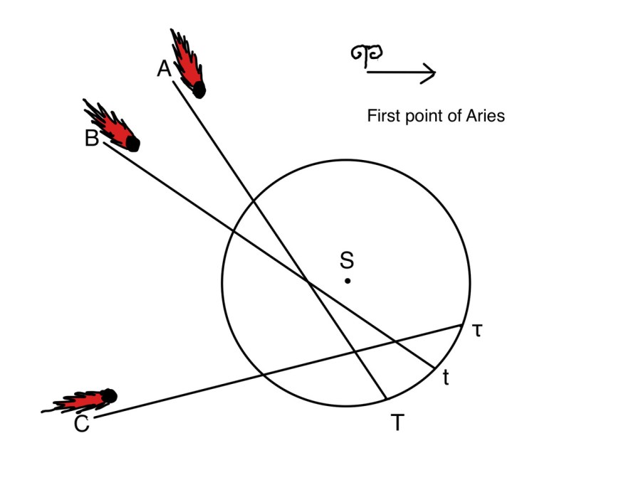
We have, as in my previous blog, placed the earth in its positions T and t and τ when these observations were made, and the lines TA and tB and τC on which we know that the phantom comet lies at the times of these observations. We would like A and B and C to be the actual positions of the phantom comet, but we do not know the distances of this comet from the earth at the appropriate times. If we can determine the true positions of A and B and C we know the corresponding positions of the real comet, as we know the latitude. These three positions determine the plane of the comet, which must pass through the sun. The orbit of the comet is then the unique conic in this plane passing through the three known positions of the comet, and with the sun at a focus.
Newton has considered the problem of determining this conic in the scholium to Proposition 21 of Section 4, Book 1.
We shall see later that if we can make a reasonably accurate estimate of the positions of the three points A and B and C, or in fact of any two of them, then we can calculate their positions as accurately as the observations will allow by successive approximation.
The question arises as to how accurate is accurate enough. We can hope to guess the position of one of A and B and C without being too far off, but two guesses would be a bridge too far. But as we only need, in the first place, an approximation to the orbit, and the orbit of the comet is approximately a parabola, we simplify the calculation by assuming that it is a parabola.
The projection of a parabola onto a plane is again a parabola, but the focus of the original parabola does not, in general, project onto the focus of the new parabola. But remember that Kepler’s second law states that comets (or rather planets), with a straight line from the comet to the sun, sweep out equal areas in equal times. It follows that the phantom comet similarly sweeps out equal areas in equal times. We know the times of the three observations, and this gives us enough information to estimate the supposedly parabolic orbit of the phantom comet, given the position of one of the points A and B and C. Now one guess suffices.
So the first step is to guess the position of B, and to compute the corresponding positions of A and C.

Having found A and C, that part of the diagram that lies to the left of AB is constructed, and the line PN gives a measure of the failure of the plane defined by the true comet when the phantom comet is at A, B and C (remember that we have the corresponding latitudes of the true comet) to pass through the sun. I omit the details of how A and C and PN are constructed. The main cause of the failure of the above plane to pass through the sun will generally be due to the inaccurate guess of the position of B. The lines GC and AF are then drawn, equal to the `error line’ .
Now repeat the construction twice, with different different choices b and β for B, and compute first the corresponding positions a and α for A, and b and κ for C, and then the corresponding measures gc and κγ; and fa and φα; for the failure of the corresponding three positions of the true comet to lie on a plane through the sun.
As the position of B varies, through the initial choice of B to b and β, the measure of the error varies through GC = FA, and gc = fa, and γκ = φα. So if smooth curves through G and g and γ, and through F and f and φ, meet the lines τC and TA in Z and X then these points are approximately the correct positions of A and C. Newton takes this curve to be a semi-circle. Unless I have missed something, this is an odd choice.
From X and Z we can compute the approximate positions of the true comet at the corresponding times, and hence determine the orbit of the comet to a reasonable degree of accuracy, as observed earlier. This orbit will probably not be a parabola, so the assumptions made in constructing this orbit are only approximately valid.
Now Newton takes three well-spaced observations of the comet. The reasons for taking different observations from those that have just been used are rather subtle. This gives three positions of the comet on its newly approximated orbit, and the condition that it sweeps out equal areas in equal times gives rise to two equations, let us call them the Kepler equations, which will not be satisfied precisely because the plane of the comet’s orbit has only been calculated approximately.
This plane is determined by two angles, as it must pass through the sun. One is the angle between the line of intersection of this plane with the plane of the ecliptic makes and the first point of Aries. The second is the angle between the two planes. Keeping either of these angles fixed, make a small change in the other, and repeat the calculation. For small changes in these angles, the effect on the Kepler equations will be linear in the small changes, and we end up two simultaneous linear equations in the corrections to the two angles. Solving these equations gives the correct changes to be made, to a good degree of accuracy.
I was intending to give the details of the construction of Newton’s diagram, but this blog is long enough and technical enough as it stands. I hope that it gives some idea of the strategic ideas, and the subtlety of the algorithm. Anyone wishing to carry out the algorithm for themselves is welcome to ask me for details. I would really like someone to give it a try. Could you have predicted the return of Halley’s comet every seventy five years?
Having done all this work, one should calculate the position of the comet at the date of every recorded observation, and compare this with the actual observation, and Newton does this.
Newton makes some observations about how he constructed his diagram. He used `tables of natural sines’, and scaled the radius of the earth’s orbit to 16 1/3 English inches. The reference to English inches points to the fact that there was quite a bewildering array of English and French feet in Newton’s time. Even at this scale, I think he must have worked to an accuracy of about a hundredth of an inch.
Observe the attention to detail of the picture that heads this blog. Newton was left
handed, a trait for which he was bullied. My next blog, in a change of direction, will look at Newton’s theology.
Charles Leedham-Green
C.R.Leedham-Green@qmul.ac.uk
Follow me on Twitter
My new translation of The Principia is published by Cambridge University Press
To get a 30% discount, visit cupbookshop.co.uk and enter the code NEWTON30 at checkout. Offer valid until 31 May 2022.

One thought on “Newton and the orbit of comets part 2”